// Twitter Cards // Prexisting Head The Biologist Is In

Friday, December 30, 2022

The Color of Beans 2

A few years back I wrote a short post to introduced a project I had started to breed up a nicely blue colored dry bean. 

https://the-biologist-is-in.blogspot.com/2018/10/the-color-of-beans-1.html

The project as been moving forward nicely since then. This year's crop was very consistently blue in color, the first time I didn't harvest a large fraction of tan/blue seeds as well.

Dry beans in mixed colors. Browns, blues, and dark greys.
The picture at left looks very similar to the one I included in the post linked above, but this photo is from a few days ago. These beans are the extras I had saved from earlier generations, including many from 2018. This tells me the best blue colored seeds are able to maintain their color well in long-term storage.

The other truly blue varieties I have come across all seem to darken towards brown during storage. "San Berdardo Blue" and the rarer "Pragerhof" beans both have a nice blue color at harvest, but that color doesn't last. My blues keeping their color for a few years in storage is a nice improvement.

Over the first several years, I selected the best blue colored seeds from each harvest to plant the following spring. Until this year's harvest, each year I kept finding brown/tan seeds. This tells me the brown color was due to recessive alleles, which means it can be very hard to filter out the brown-seed trait. Any given blue seed could be hiding the recessive brown color allele.

Dark blue dry beans.
This year I was lucky and the entire harvest had the rich blue color I had been working towards. The recessive allele for brown color could still be hiding among these. I won't be more certain I have finished filtering out that trait for at least a couple more years, but I am hopeful. Because I didn't have to select on color this year, I instead selected for larger seed size and pods (or pod clusters) with more seeds in them.

Right now I am working to figure out how I can distribute this new variety, but it may not happen this year. I have very limited seed stock and any method of selling or distributing them comes with some significant costs.

You can find more about these beans with the tag #BlueBeanProject on various social media systems. I'll also be writing more posts here, so stay tuned.


Eleven pale blue bean seeds, each with a black ring around the hilium.Five dark blue bean seeds with tan speckles.
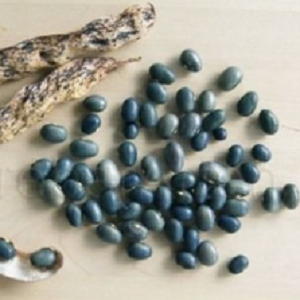
I also have a couple new blue lines, unrelated to those above. These samples are F2s from a cross between "Pragerhof" and an unknown black bean.

One blue is darker than my main line and the other is lighter. I don't know for sure what these will become during the several years it will take to stabilize their genetics, but I aim to find out!

References:

Thursday, May 20, 2021

Viable Interspecific Eggplant Hybrids

The last year has been a mess. I'm fine. My family is fine. Most of my friends are fine. The increased anxiety and stress basically shut off any motivation or ability I had to write posts here. I was still active over on twitter or instagram, as those require less focused thought, but I just couldn't will myself to sit down at a computer and type up anything I felt was worthwhile to post.

I'm now fully vaccinated against covid19, but I know there are many people who still have not been able to access a vaccine. Some in my family. Many in the broader community. Covid cases in my community are dropping, but they're still higher than the peak we had in May of last year. I worry about recent CDC guidance and how people broadly seem to think it means the pandemic is over. It is not. Not here, and not elsewhere.

For now, most people locally seem to still be keeping up distancing and masking practices gained over the last year. As always, the next few weeks will be informative.

Even with the persistent writer's block, I routinely thought about writing something. This post is the first something to come of that. It isn't really the long and information or photo rich posts I like to write, but it is what it is


My plant breeding projects have continued without interruption. My gardens have provided me with useful exercise and amusement.

Most of my plant breeding projects start with hybrids between divergent varieties within one species. The F1 generally stands out from the two parental lines, so Iit is fairly easy to have confidence that the cross took. In the F2 generation, there are almost always useful and unexpected traits which segregates out.

Last year I grew out a F2 population of scarlet eggplant. Every plant was different, but two stood out. One was extra productive and ripened fruit far earlier than any others. The other developed fruit that were white when immature, but ripened to the typical red later. This season I have F3 populations from those two plants.

I still haven't figured out how to like eating eggplant, especially the more bitter flavors of the scarlet eggplant, but I like the plants and will continue to try.

Recently I found some references describing successful hybrids between the scarlet eggplant (Solanum aethiopicum) and more common purple eggplant (S. melongena), with some significant effort in the lab. This got me thinking about what species one could make hybrids with among the eggplant. Any such hybrids would allow for much more diverse F2 populations, with their higher potential for selection towards interesting new traits.

This led to some discussion about primary (1'), secondary (2'), and tertiary (3') germplasm. 1' germplasm includes plants in the same or related species which can cross readily to your subject species. 2' germplasm includes plants which can cross to your subject species with significant reduction in fertility. 3' germplasm is then plants that can cross with your subject only with intensive laboratory operations such as embryo rescue or induced genome duplication.

In the case of eggplants, there has been much more exploration of 2' and 3' germplasm for the common eggplant. The scarlet eggplant is an important crop for many communities, but it has not attracted as much attention in communities with higher levels of biological research investment. As such, the 2' and 3' germplasm lists below for scarlet eggplant are very much incomplete.

 Asian Eggplant (Solanum melongena)

  1. primary: S. incanum and S. insanum.
  2. secondary: S. anguivi, S. dasyphyllum, S. lichtensteinii, S. linnaeanum, S. pyracanthos, S. tomentosum, and S. violaceum.
  3. tertiary: S. elaeagnifolium, S. sisymbriifolium, S. torvum, and S. aethiopicum.

Scarlet Eggplant (Solanum aethiopicum)

  1. primary: S. anguivi, S. macrocarpon, and S. dasyphyllum
  2. secondary:
  3. tertiary: S. melongena.

Professional plant breeders pursue traits from related species like these to improve disease resistance, drought resistance, or other traits important to growing large crops.

Independent plant breeders can afford to use traits from related species (among the 1' and 2' germplasm resources at least) to express their creativity towards developing new varieties. Even if you're not sure what to do with them (as I am), they're still lovely plants which might be fun to work with in the garden.

I hope you are and remain well as the pandemic continues.


References

Friday, February 21, 2020

Photoshop again.

Online seed vendors vary dramatically from the largely respectable, to the folks selling "peppers" like those below that I found on the Amazon or Ebay marketplaces.

To you, the botanically savvy purchaser, these vendors stand out as clearly fraudulent. But not everyone is botanically savvy. People who don't instantly know these wonderful colored peppers are just photoshopped versions of a red pepper photo are such vendors intended "customers".

Pile of cayenne peppers photo edited to look cyan in color. Pile of cayenne peppers photo edited to look blue in color. Pile of cayenne peppers photo edited to look purple in color. Pile of cayenne peppers photo edited to look magenta in color. Pile of cayenne peppers; original photo the others here were modified from.


Even among the largely respectable vendors, there are a wide range of philosophical or political stances that may impact your decisions of who to buy from. Does the company support white supremacists? Do they sell patented plant varieties? Do they push pseudo-science in their catalogs?

It can take some digging to be certain you agree with the politics behind any given company. It can take significant effort to bring such considerations into your buying decisions, so I understand if you choose not to do so.

But please, don't buy seeds from vendors selling off-hue peppers, blue strawberries, rainbow roses, rainbow onions, or the many other scams that are out there. If something looks too good to be true, at the very least investigate further. These online vendors rely on people clicking "buy" when seeing something interesting. By the time you've grown up the seeds and realize you were scammed, the time to contest the purchase in the marketplaces the vendors work through will have long since expired.

Friday, February 14, 2020

Tomatillo Breeding (4/n)

The last couple posts have looked at simulations for selection of a single gene, for recessive or dominant alleles. Increasing the number of genes actively under selection results in it taking longer and longer for the population to converge.
Plot titled "Multiple recessive traits, large population", illustrating selection for a trait in an out-crossing population.
Plot titled "Multiple dominant traits, large population", illustrating selection for a trait in an out-crossing population. It takes more years for the trait of interest to reach saturation in the population.
The change in code to simulate multiple genetic loci is really simple if we assume the different alleles we're selecting on are found sufficiently distant from each other on the chromosomes. This is referred to as "un-linked" and means the probability calculations for each are independent of the others.

R Script 5: Multiple recessive traits, large population.
# One recessive trait, infinite population.
#     Stabilize progeny for recessive trait via selection.
#     Save seeds from double-recessive plants each generation.
years <- 10;

# Define F2 population.
P_AA <- vector();
P_Aa <- vector();
P_aa <- vector();
P_AA <- 0.25;
P_Aa <- 0.50;
P_aa <- 0.25;

# Save seeds only from aabb plants, unknown pollen donor. Iterate over years.
for(i in 1:years) {
  P_AA <- append(P_AA,   0);
  P_Aa <- append(P_Aa,   P_aa[i]*P_AA[i]*1.00 + P_aa[i]*P_Aa[i]*0.50);
  P_aa <- append(P_aa,   P_aa[i]*P_aa[i]*1.00 + P_aa[i]*P_Aa[i]*0.50);
  P_sum <- P_aa[i+1] + P_Aa[i+1];
  P_Aa[i+1] <- P_Aa[i+1]/P_sum;
  P_aa[i+1] <- P_aa[i+1]/P_sum;
}

# Make figure.
plot(  0:years, P_aa^1, col="red", main="Multiple recessive traits, large population.", xlab="Years", ylab="%aa pollen donors", xlim=c(0,years), ylim=c(0,1), axes=TRUE, frame.plot=TRUE);
lines(0:years, P_aa^1, col="red");
lines(0:years, 1-P_aa^1, col="blue", lty="dashed");
lines(c(0,years),c(0.95,0.95), col="black", lty="dotted");
lines(c(0,years),c(0.99,0.99), col="black", lty="dashed");

for(i in 2:20) {
  lines(0:years, P_aa^i, col="red");
  lines(0:years, 1-P_aa^i, col="blue", lty="dashed");
}

R Script 6: Multiple dominant traits, large population.
# One dominant trait, infinite population.
#     Stabilize progeny for dominant trait via selection.
#     Save seeds from dominant plants each generation.
years <- 10;

# Define F2 population.
P_AA <- vector();
P_Aa <- vector();
P_aa <- vector();
P_AA <- 0.25;
P_Aa <- 0.50;
P_aa <- 0.25;

# Save seeds only from (AA and Aa) plants, unknown pollen donor. Iterate over years.
for(i in 1:years) {
  P_AA <- append(P_AA,   P_AA[i]*P_AA[i]*1.00 + P_AA[i]*P_Aa[i]*0.50 + P_Aa[i]*P_Aa[i]*0.25);
  P_Aa <- append(P_Aa,   P_AA[i]*P_aa[i]*1.00 + P_AA[i]*P_Aa[i]*0.50 + P_Aa[i]*P_aa[i]*0.50 + P_Aa[i]*P_Aa[i]*0.50);
  P_aa <- append(P_aa,   0);
  
  P_sum <- P_AA[i+1] + P_Aa[i+1];
  P_AA[i+1] <- P_AA[i+1]/P_sum;
  P_Aa[i+1] <- P_Aa[i+1]/P_sum;
}

# Make figure.
plot(  0:years, P_AA, col="red", main="Multiple dominant traits, large population.", xlab="Years", ylab="%AA pollen donors", xlim=c(0,years), ylim=c(0,1), axes=TRUE, frame.plot=TRUE);
lines(0:years, P_AA, col="red");
lines(0:years, 1-P_AA, col="blue", lty="dashed");
lines(c(0,years),c(0.95,0.95), col="black", lty="dotted");
lines(c(0,years),c(0.99,0.99), col="black", lty="dashed");

for(i in 2:20) {
  lines(0:years, P_AA^i, col="red");
  lines(0:years, 1-P_AA^i, col="blue", lty="dashed");
}


The probability of an F2 plant having two copies of recessive alleles for multiple genes drops to minimal very quickly when we increase the number of genes. In a small population this low probability means we might not find an F2 with all the recessive alleles stacked up the way we might want. All is not lost.

With our small F2 population, roughly a quarter would be expected to be in the double-recessive condition for the first gene of interest.

25% AA; 50% Aa; 25% aa

If we were unlucky and couldn't find a single plant that was also double-recessive for the second gene of interest, we can go ahead with plants showing the dominant trait for that second gene. The probability is that two thirds of the plants showing the dominant trait for the second gene will be heterozygous, carrying one copy of the recessive allele.

aaB_ (⅓BB; ⅔Bb)

In the next generation we have pretty good odds of recovering that second recessive trait that we were looking for. This way we can progressively collect multiple recessive traits without finding them in that first F2 generation. With this strategy, we need to keep seeds from prior generations. If we can't recover that next recessive trait in the next year, then we managed to find plants that were not heterozygous for the gene of interest. We need to grow more plants from the previous generation again, to try and find some carrying a copy of the recessive allele.


With plants that typically self-pollinate (like peppers and tomatoes), it can be pretty simple to intentionally remove recessive alleles for genes of interest. If you grow out the seeds produced by a plant and find any double-recessive progeny, you know that plant was heterozygous. If you don't find any double-recessive progeny, if you grow enough seeds, you can be pretty confident of that plant being homozygous for the dominant allele.

With plants that can't self-pollinate (like tomatillos), it can take more work/time. Lets say we have one plant that is showing the dominant trait. If we cross it with a plant showing the recessive trait, the resulting progeny will tell us if that first plant is "AA" or "Aa". If all the progeny show the dominant trait, then the plant we were testing is "AA". If the progeny show a mix of dominant and recessive traits, then the plant we were testing is "Aa" (and can be discarded). This is called a "test-cross" because it is used to test the genetics of a specific individual, even though we have no interest in using the progeny that result for further breeding work.

Since tomatilloes can be kept alive over several years, you can use such test crosses to progressively collect multiple plants with just the dominant alleles for your genes of interest. Once you have a few such plants, you can then allow them to inter-cross and be confident you won't have the recessive allele turning up in the next generations.

Friday, February 7, 2020

Tomatillo Breeding (3/n)

I've been doing some math to help me think about breeding strategies with tomatillos. Last week I showed some code for calculating how populations of different sizes converge under selection for a single recessive trait. Here I'll show similar code for a single dominant trait.


X-axis, years going from 0 to 10. Y-axis, "%AA pollen donors" going from 0 to 1. Red curve for %AA goes from lower left, rises slowly towards 1, and then smooths out to approach 1. Blue curve descends in a mirror image.
Solid red curve with circles: %AA pollen donors.
Dashed blue curve: %Aa & %aa pollen donors.
Like before, we'll start with an infinite population.

Since we can't tell the difference between plants with one or two copies of the dominant trait ("AA" or "Aa"), we can't tell what the genetic status is of any one plant that we save seeds from. Our goal is a population entirely consisting of "AA" plants, so that is what the code will plot.

The zero year is our F2 population. It takes seven years for the "AA" individuals to represent 95% (dotted horizontal line) of the population. Three years later the level crosses above 99% (dashed horizontal line) of the population.

Because this is the infinite population scenario, there will always be a small percentage of the population carrying the recessive allele.

R Script 3: One dominant trait, infinite population.
# One dominant trait, infinite population.
#     Stabilize progeny for dominant trait via selection.
#     Save seeds from dominant plants each generation.
years <- 10;

# Define F2 population.
P_AA <- vector();
P_Aa <- vector();
P_aa <- vector();
P_AA <- 0.25;
P_Aa <- 0.50;
P_aa <- 0.25;

# Save seeds only from (AA and Aa) plants, unknown pollen donor. Iterate over years.
for(i in 1:years) {
  P_AA <- append(P_AA,   P_AA[i]*P_AA[i]*1.00 + P_AA[i]*P_Aa[i]*0.50 + P_Aa[i]*P_Aa[i]*0.25);
  P_Aa <- append(P_Aa,   P_AA[i]*P_aa[i]*1.00 + P_AA[i]*P_Aa[i]*0.50 + P_Aa[i]*P_aa[i]*0.50 + P_Aa[i]*P_Aa[i]*0.50);
  P_aa <- append(P_aa,   0);
  
  P_sum <- P_AA[i+1] + P_Aa[i+1];
  P_AA[i+1] <- P_AA[i+1]/P_sum;
  P_Aa[i+1] <- P_Aa[i+1]/P_sum;
}

# Make figure.
plot(  0:years, P_AA, col="red", main="One dominant trait, large population.", xlab="Years", ylab="%AA pollen donors", xlim=c(0,years), ylim=c(0,1), axes=TRUE, frame.plot=TRUE);
lines(0:years, P_AA, col="red");
lines(0:years, P_Aa+P_aa, col="blue", lty="dashed");
lines(c(0,years),c(0.95,0.95), col="black", lty="dotted");
lines(c(0,years),c(0.99,0.99), col="black", lty="dashed")

X-axis, years going from 0 to 10. Y-axis, "%target Pollen Donors" going from 0 to 1. Cyan curve for recessive percentage goes from lower left, rises sharply towards 1, and then smooths out to approach 1. Red curve for dominant percentage goes from lower left, rises slowly towards 1, and then smooths out to approach 1. Yellow curve descends in a mirror image of cyan curve. Blue curve descends in a mirror image of red curve.
Cyan line w/circles: recessive selection.
Red line w/circles: dominant selection.
To compare the trajectory for selection on the recessive allele vs on the dominant allele, I overlaid the two curves in an image editor. I inverted the colors for the recessive curves to better distinguish them from the added dominant curves.

Selection on a dominant trait progresses at a slower rate initially than selection on a recessive trait, but by about ten years the two approaches would be expected to reach a similar degree of completeness.

With smaller population sizes, we'd expect the selected allele (dominant or recessive) to reach complete saturation by about that time point.


With recessive traits, I only had to consider "aa" plants as seed producers. With dominant traits, I have to consider "AA" and "Aa" plants. This seems like a small difference, but for simulating small numbers this adds significant complexity.

Similar to above figure, but each curve is replaced by a tight cluster of overlapping curves representing individual runs of the simulation.
Population = 1000
Similar to above figure, but each curve is replaced by a very loose cluster of overlapping curves representing individual runs of the simulation.
Population = 50
Similar to above figure, but each curve is replaced by an extremely loose cluster of overlapping curves representing individual runs of the simulation. These curves occupy almost the entire figure.
Population = 10

If you compare these plots to those for the recessive selection scenario (https://the-biologist-is-in.blogspot.com/2020/01/tomatillo-breeding-2n.html), you'll see that this scenario has a much higher level of noise in the trajectories. For the smallest population level, it takes 30 years (not shown in figures) for the majority of the experimental replicates to converge on the targeted "AA" condition.

R Script 4: One dominant trait, small population.
# One dominant trait, small population.
#     Stabilize progeny for dominant trait via selection.
#     Save seeds from dominant plants each generation.
years <- 10;
population <- 1000; # 1000, 50, 10
trials <- 100;

# Intialize figure.
plot( c(0,years),c(0,years), col="red", main="One dominant trait, small population.", xlab="Years", ylab="%AA pollen donors", xlim=c(0,years), ylim=c(0,1), axes=TRUE, frame.plot=TRUE);
lines(c(0,years),c(0.95,0.95), col="black", lty="dotted");
lines(c(0,years),c(0.99,0.99), col="black", lty="dashed");

for (ii in 1:trials) {
  # Define F2 population probabilities for selection on AA plants.
  P_AA_1 <- vector();
  P_Aa_1 <- vector();
  P_aa_1 <- vector();
  P_AA_1 <- 0.25;
  P_Aa_1 <- 0.50;
  P_aa_1 <- 0.25;
  
  # Define F2 population probabilities for selection on Aa plants.
  P_AA_2 <- vector();
  P_Aa_2 <- vector();
  P_aa_2 <- vector();
  P_AA_2 <- 0.25;
  P_Aa_2 <- 0.50;
  P_aa_2 <- 0.25;

  # Save seeds only from (AA and Aa) plants, which can't self-polinate.
  for (i in 1:(years+2)) {
    # Generate actual population.
    rands <- runif(population, 0, 1);
    Genotypes <- vector();
    for (j in 1:population) {
      if (rands[j] < P_AA_1[i]) {
        Genotypes <- append(Genotypes, "AA");
      } else if (rands[j] < P_AA_1[i]+P_Aa_1[i]) {
        Genotypes <- append(Genotypes, "Aa");
      } else {
        Genotypes <- append(Genotypes, "aa");
      }
    }
    Genotype_counts <- table(Genotypes);
    
    # Determine actual genotype probabilities for pollen donors. (Assuming "AA" plant in case 1, "Aa" plant in case 2.)
    if (is.na(Genotype_counts["AA"])) {
      P_AA_1[i] <- 0;
      P_AA_2[i] <- 0;
    } else {
      P_AA_1[i] <- (Genotype_counts["AA"]-1)/(population-1); # The plant we're saving seeds from can't be polinated by itself.
      P_AA_2[i] <- Genotype_counts["AA"]/(population-1);
    }
    if (is.na(Genotype_counts["Aa"])) {
      P_Aa_1[i] <- 0;
      P_Aa_2[i] <- 0;
    } else {
      P_Aa_1[i] <- Genotype_counts["Aa"]/(population-1);
      P_Aa_2[i] <- (Genotype_counts["AA"]-1)/(population-1); # The plant we're saving seeds from can't be polinated by itself.
    }
    if (is.na(Genotype_counts["aa"])) {
      P_aa_1[i] <- 0;
      P_aa_2[i] <- 0;
    } else {
      P_aa_1[i] <- Genotype_counts["aa"]/(population-1);
      P_aa_2[i] <- Genotype_counts["aa"]/(population-1);
    }
  
    # Generate new theoretical genotype probabilities.
    P_AA_1 <- append(P_AA_1,   P_AA_1[i]*P_AA_1[i]*1.00 + P_AA_1[i]*P_Aa_1[i]*0.50 + P_Aa_1[i]*P_Aa_1[i]*0.25);
    P_Aa_1 <- append(P_Aa_1,   P_AA_1[i]*P_aa_1[i]*1.00 + P_AA_1[i]*P_Aa_1[i]*0.50 + P_Aa_1[i]*P_aa_1[i]*0.50 + P_Aa_1[i]*P_Aa_1[i]*0.50);
    P_aa_1 <- append(P_aa_1,   0);
    
    P_AA_2 <- append(P_AA_2,   P_AA_2[i]*P_AA_2[i]*1.00 + P_AA_2[i]*P_Aa_2[i]*0.50 + P_Aa_2[i]*P_Aa_2[i]*0.25);
    P_Aa_2 <- append(P_Aa_2,   P_AA_2[i]*P_aa_2[i]*1.00 + P_AA_2[i]*P_Aa_2[i]*0.50 + P_Aa_2[i]*P_aa_2[i]*0.50 + P_Aa_2[i]*P_Aa_2[i]*0.50);
    P_aa_2 <- append(P_aa_2,   0);

    P_sum_1 <- P_AA_1[i+1] + P_Aa_1[i+1];
    P_AA_1[i+1] <- P_AA_1[i+1]/P_sum_1;
    P_Aa_1[i+1] <- P_Aa_1[i+1]/P_sum_1;
    
    P_sum_2 <- P_AA_2[i+1] + P_Aa_2[i+1];
    P_AA_2[i+1] <- P_AA_2[i+1]/P_sum_2;
    P_Aa_2[i+1] <- P_Aa_2[i+1]/P_sum_2;
    
    # Weighted average of the two probability sets by proportion of "AA" vs "Aa" plants.
    #  Only _1 values carry over to next iteration.
    if (is.na(Genotype_counts["AA"])) {
      count_AA <- 0; } else {
      count_AA <- Genotype_counts["AA"];
    }
    if (is.na(Genotype_counts["Aa"])) {
      count_Aa <- 0; } else {
      count_Aa <- Genotype_counts["Aa"];
    }
    weight1 <- count_AA/(count_AA+count_Aa);
    weight2 <- 1-weight1;
    val_AA_1 <- P_AA_1[i+1];
    val_AA_2 <- P_AA_2[i+1];
    val_Aa_1 <- P_Aa_1[i+1];
    val_Aa_2 <- P_Aa_2[i+1];
    P_AA_1[i+1] <- val_AA_1*weight1 + val_AA_2*weight2;
    P_Aa_1[i+1] <- val_Aa_1*weight1 + val_Aa_2*weight2;
    
    if (is.na(P_AA_1[i+1]) == TRUE) {  P_AA_1[i+1] <- 0;  }
    if (is.na(P_Aa_1[i+1]) == TRUE) {  P_Aa_1[i+1] <- 0;  }
    
    if ((P_AA_1[i+1]+P_Aa_1[i+1]) == 0) {
      # End simulation cycle if no "AA" or "Aa" plants.
      for (j in (length(P_aa_1)):years) {
        P_AA_1 <- append(P_AA_1,   0);
        P_Aa_1 <- append(P_Aa_1,   0);
        P_aa_1 <- append(P_aa_1,   0);
      }
      break;
    }
    
    ## Debugging output.
    #message("Iteration ", i);
    #print(Genotypes);
    #message("  ");
  }

  # Add current simulation cycle to figure.
  points(0:years, P_AA_1[1:(years+1)], col="red");
  lines( 0:years, P_AA_1[1:(years+1)], col="red");
  lines( 0:years, 1-P_AA_1[1:(years+1)], col="blue", lty="dashed");
}


This essentially means it isn't possible to selectively breed a dominant trait to complete saturation in a small population just using simple selection.

Unlike in the recessive case, we can't just save a few plants over winter to reset the population with only the exact genetics we want. A similar strategy should allow for more rapid progress towards the goal, however.

I'll explore this topic further next time.

Friday, January 31, 2020

Tomatillo Breeding (2/n)

I thought it would take me a week to get back to this, but that didn't happen. Oops. Sorry.


The big difficulty with tomatillo breeding is that they're very strong out-crossers. Unlike tomatoes, peppers, eggplant, beans, etc., you can't just grow one plant from each generation to help reduce control the genetics during the process of making a new variety. If you grow a dozen tomatillo plants and don't like how half of them grew, you can be sure that seeds saved from the plants you liked will have genetics from the ones you didn't.

I worked out some of the math long-hand, showing how this difficulty plays out over several generations. I faltered when it came to the task of outlining all those calculations via text. It is easy enough to throw a few equations into text, but I didn't want to post pages of derivations for you to read through. (And I'd have most assuredly made silly typos along the way.)

Instead, I wrote up some simulations in R. These can be run using RStudio if you want to play around with them, or you can just look at my summary figures here.


X-axis, years going from 0 to 10. Y-axis, "%aa pollen donors" going from 0 to 1. Red curve for %aa goes from lower left, rises rapidly towards 1, and then smooths out to approach 1. Blue curve descends in a mirror image.
Solid red curve with circles: %aa pollen donors.
Dashed blue curve: %Aa & %AA pollen donors.
We'll start with the simple case of a single recessive trait in an infinite population. (Sometimes infinity makes the math hard to do, other times it makes it very easy.)

If we seeds only from plants showing the recessive trait, we can rapidly select away the dominant allele. The zero year of this plot is the F2 generation, where traits first start assorting. It takes five years for the recessive trait to be at 95% (dotted horizontal line) of the population and another three for it to be at 99% (dashed horizontal line) of the population.

Because the population is infinite, we can never quite reach 100%. There will always be a small amount of the dominant allele hanging around.

R Script 1: One recessive trait, infinite population.
# One recessive trait, infinite population.
#     Stabilize progeny for recessive trait via selection.
#     Save seeds from double-recessive plants each generation.
years <- 10;

# Define F2 population.
P_AA <- vector();
P_Aa <- vector();
P_aa <- vector();
P_AA <- 0.25;
P_Aa <- 0.50;
P_aa <- 0.25;

# Save seeds only from aa plants, unknown pollen donor. Iterate over years.
for(i in 1:years) {
  P_AA <- append(P_AA,   0);
  P_Aa <- append(P_Aa,   P_aa[i]*P_AA[i]*1.00 + P_aa[i]*P_Aa[i]*0.50);
  P_aa <- append(P_aa,   P_aa[i]*P_aa[i]*1.00 + P_aa[i]*P_Aa[i]*0.50);
  P_sum <- P_aa[i+1] + P_Aa[i+1];
  P_Aa[i+1] <- P_Aa[i+1]/P_sum;
  P_aa[i+1] <- P_aa[i+1]/P_sum;
}

# Make figure.
plot(  0:years, P_aa, col="red", main="One recessive trait, large population.", xlab="Years", ylab="%aa pollen donors", xlim=c(0,years), ylim=c(0,1), axes=TRUE, frame.plot=TRUE);
lines(0:years, P_aa, col="red");
lines(0:years, P_Aa+P_AA, col="red", lty="dashed");
lines(c(0,years),c(0.95,0.95), col="black", lty="dotted");
lines(c(0,years),c(0.99,0.99), col="black", lty="dashed")


We can extend this simulation to better model a realistic situation where you can only grow a limited number of plants. Coding this is much more complicated. If we run it with a large population, we see a pattern much like the infinite one above. If we run it with a small population, we get very noisy trajectories that vary a lot from run to run. At small population numbers, it is fairly easy to accidentally end the experiment with no "aa" plants to save seeds from. (In real life, we'd just go back to seeds from the previous generation.)

Similar to above figure, but each curve is replaced by a tight cluster of overlapping curves representing individual runs of the simulation.
Population = 1000
Similar to above figure, but each curve is replaced by a loose cluster of overlapping curves representing individual runs of the simulation.
Population =50
Similar to above figure, but each curve is replaced by a very loose cluster of overlapping curves representing individual runs of the simulation. The curves are so noisy that the cluster is spread over much of the plot.
Population =10

The upshot of the simulations is that if we grow small numbers of plants each generation, we can eventually eliminate the pesky dominant alleles for the trait of interest. It will take a while, but it is doable if you're willing to wait several years to a decade.

R Script 2: One recessive trait, small population.
# One recessive trait, small population.
#     Stabilize progeny for recessive trait via selection.
#     Save seeds from double-recessive plants each generation.
years <- 10;
population <- 50; # 1000, 50, 10
trials <- 100;

# Intialize figure.
plot(  c(0,years),c(0,years), col="red", main="One recessive trait, small population.", xlab="Years", ylab="%aa pollen donors", xlim=c(0,years), ylim=c(0,1), axes=TRUE, frame.plot=TRUE);
lines(c(0,years),c(0.95,0.95), col="black", lty="dotted");
lines(c(0,years),c(0.99,0.99), col="black", lty="dashed");

for (ii in 1:trials) {
  # Define F2 population probabilities
  P_AA <- vector();
  P_Aa <- vector();
  P_aa <- vector();
  P_AA <- 0.25;
  P_Aa <- 0.50;
  P_aa <- 0.25;

  # Save seeds only from "aa" plants, which can't self-polinate.
  for (i in 1:(years+2)) {
    # Generate actual population.
    rands <- runif(population, 0, 1);
    Genotypes <- vector();
    for (j in 1:population) {
      if (rands[j] < P_AA[i]) {
        Genotypes <- append(Genotypes, "AA");
      } else if (rands[j] < P_AA[i]+P_Aa[i]) {
        Genotypes <- append(Genotypes, "Aa");
      } else {
        Genotypes <- append(Genotypes, "aa");
      }
    }
    Genotype_counts <- table(Genotypes);
    
    # Determine actual genotype probabilities for pollen donors.
    if (is.na(Genotype_counts["AA"])) {
      P_AA[i] <- 0; } else {
      P_AA[i] <- Genotype_counts["AA"]/(population-1);
    }
    if (is.na(Genotype_counts["Aa"])) {
      P_Aa[i] <- 0; } else {
      P_Aa[i] <- Genotype_counts["Aa"]/(population-1);
    }
    if (is.na(Genotype_counts["aa"])) {
      P_aa[i] <- 0; } else {
      P_aa[i] <- (Genotype_counts["aa"]-1)/(population-1); # The plant we're saving seeds from can't be polinated by itself.  
    }
  
    # Generate new theoretical genotype probabilities.
    P_AA <- append(P_AA,   0);
    P_Aa <- append(P_Aa,   P_aa[i]*P_AA[i]*1.00 + P_aa[i]*P_Aa[i]*0.50);
    P_aa <- append(P_aa,   P_aa[i]*P_aa[i]*1.00 + P_aa[i]*P_Aa[i]*0.50);
    
    P_sum <- P_aa[i+1] + P_Aa[i+1];
    P_Aa[i+1] <- P_Aa[i+1]/P_sum;
    P_aa[i+1] <- P_aa[i+1]/P_sum;
    
    if (is.na(P_Aa[i+1]) == TRUE) {  P_Aa[i+1] <- 0;  }
    if (is.na(P_aa[i+1]) == TRUE) {  P_aa[i+1] <- 0;  }
    
    if (P_aa[i+1] == 0) {
      # End simulation cycle if no "aa" plants.
      for (j in (length(P_aa)):years) {
        P_AA <- append(P_AA,   0);
        P_Aa <- append(P_Aa,   0);
        P_aa <- append(P_aa,   0);
      }
      break;
    }
  }

  # Add current simulation cycle to figure.
  points(0:years, P_aa[1:(years+1)], col="red");
  lines( 0:years, P_aa[1:(years+1)], col="red");
  lines( 0:years, 1-P_aa[1:(years+1)], col="blue", lty="dashed");
}


However, there's a much faster way to complete the process. It might even only take a couple years.

Tomatilloes are perennial where it is warm enough for them to survive through winter. They also easily root from cuttings. These traits combined mean we can pot up rooted cuttings from each plant at the end of one year and continue growing selected plants the next year after we've had a chance to evaluate their fruit characteristics.

You'd have to grow enough plants the first year to be able to find multiple individuals with the recessive traits you're interested in. The next year, you can continue growing only those few plants and allow them to cross-pollinate. Every seed they produce in their second year will contain those recessive traits you selected the parents for. The dominant alleles will be gone from your population.

You're done in one year of selection and another for seed production. No waiting around for a decade or more, gambling with the whims of chance. You may have your new tomatillo variety complete and ready to go.


I didn't talk about dominant traits here. They're a bit more involved and I'll have to do another post about that case. I'll also have to do another post talking about the case where you're looking for multiple specific genes (recessive or dominant) at once.

It looks like my planned two part series is going to be a bit longer in the end.

Thursday, December 5, 2019

Tomatillo Breeding (1/n)

Tomatillos are a wonderful vegetable plant to grow. There are several distinct varieties available, but nowhere near the numbers we see for tomatoes, peppers, or other crops. What's the difference?

Tomatillos are almost exclusively out-breeders. You need two or more plants growing in an area to get good production of fruit. As a result, every plant is a new hybrid and a population will maintain a high degree of genetic diversity. This also makes it difficult for different varieties to be grown in the same area, as they will generally cross and meld into one diverse population.


A few years back I started an experiment with breeding tomatillos. I grew one plant of a variety with small purple fruit next to one plant of a variety with large green fruit. I had saved seeds from a CSA and the local grocer, so I don't have any specific variety names to give you. (If you want to replicate the experiment, the purple variety was similar to: https://www.edenbrothers.com/store/purple-tomatillo-seeds.html; the green to: https://www.edenbrothers.com/store/rio-grande-verde-tomatillo-seeds.html.)

Four tomatillo fruit, from left to right. 1) Medium purple. 2) Small purple. 3) Large green. 4) Medium purple.
#1. Medium purple fruit.
#2. Small purple fruit.
#3. Large green fruit, with purple dots.
#4. Medium purple fruit.
Because the plants are such extreme out-crossers, every seed that year was expected to be a hybrid between the two different varieties. The next year I grew four plants, from seeds I saved from the purple plant. Each plant grew distinct fruit. (1-4, left to right in photo at right.) This diversity tells us that both parental varieties were highly heterogeneous, so the specifics of each hybrid plant depended on exactly which allele they inherited from each parent. As none of my neighbors were growing tomatillos, we can be pretty sure each one was pollinated by the other three.


Two large green tomatillo fruit at right. Six small pale purple tomatillo fruit at left.
F2s from F1#3.

The next year I planted seeds I had saved from plant #3. I grew 11 plants, but only 5 produced any fruit. The plants looked like they'd been exposed to an herbicide from the commercial garden soil I had added to the garden at the start of the season (Herbicide carryover). All the fruit were green, with some later developing some purple pigment as they ripened off the plant.

Ten bowls filled with tomatillo fruit. Contents of each bowl are different sizes and/or shades of green and purple.
F2s from F1#4.
This year I planted seeds I had saved from plant #4. I grew 12 plants and all produced fruit. These showed a much wider range of pigment levels, including a pair of plants with visible purple pigment and large fruit.

One plant had a trait I didn't like at all. The fruit from spoiled very rapidly after picking. (Previous year's fruit stored for months.) That plant was one of two in an isolated garden, so I immediately culled all of the fruit from both plants. I didn't want to risk the genetics associated with spoilage turning up in the garden again next year.

Overhead view of orange plastic bowl filled with large tomatillos. The fruit are combinations of green and dark purple. One fruit at center is mostly green with three purple stripes starting at the bottom.
One plant had fruit I really liked. The fruit were large and developed purple pigment, the traits I have been trying to combine in one plant. I wasn't expecting the fruit to develop stripes as they were maturing, however. These fruit are not lasting as long as I'd like, but the other good traits means I'll be saving seeds from them anyhow.
Overhead view of green plastic bowl filled with medium tomatillos. The fruit are dark purple, with the most ripe looking black..
A couple other plants produced intensely dark purple fruit, appearing ink-black. This is the color I've been looking for, but the fruit aren't as large as I want. I'll save seeds from these as well.

Because the plants are out-crossers, I know they will have been pollinated by the others in the garden. Even though these two have trait combinations I really like, it will be unlikely to find offspring with the same traits because of all the other traits in the garden.

I've tried to diagram the overall history of the project so far. (I didn't have any photos of the original varieties, so they get cartoon representations.)

At top are a small dark purple and large green circle, representing the original varieties I crossed. From the dark circle, a black line goes down to a second row consisting of four tomatillo fruit pictures. (From left to right: medium purple, small purple, large green, & medium purple.) Black lines are drawn from beneath the right two fruit downwards to photos. Left line goes to a photo of 5 bowls of green fruit, with a photo of pale purple fruit to the left. The right line goes to a photo of 10 bowls of fruit with varying colors of purple and green.
Tomatillo project history so far.

About this point I started thinking about how I might get around the issues caused by the potential for genes from every plant in a garden to turn up in the next generation. I don't want to have to cull everything from a garden when something strongly negative turns up in the population. Right now I only have two isolated garden spaces, so that strategy can only go so far.

For my solution, come back in a week for part 2!


References: